Next: 6 Graphical representations Up: MANOR: Micro-Array NORmalization of Previous: 4 qscore class Contents
We provide examples of array-CGH data coming from two different platforms. These data illustrate the need for appropriate within-array normalization methods, and especially the need for methods that handle spatial effects.
> data(spatial)
For each array we provide raw data (generated by Genepix or SPOT (5)), as well as the corresponding arrayCGH object before and after normalization.
These arrays illustrate the main source of non biological variability of these data sets, namely spatial effects. We classify these effects into two non exclusive types: local bias and global gradients. In the case of local bias, entire areas of the array show lower or higher signal values than the rest of the array, with no biological explanation (array edge); to our experience, this particular type of artifact roughly affects an array out of two. In the case of global gradients, the array shows an obvious signal gradient from one side of the slide to the other (array gradient).
> data(spatial) > arrayPlot(edge, "LogRatio", main = "Local spatial effects", zlim = c(-1, + 1), mediancenter = TRUE, bar = "h") 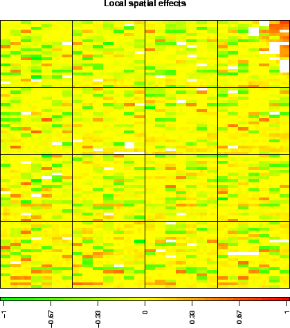 |
> data(spatial) > arrayPlot(gradient, "LogRatio", main = "Spatial gradient", zlim = c(-2, + 2), mediancenter = TRUE, bar = "h") 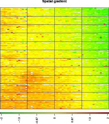 |