|
|
{xi}1m - data points for approximation.
{yi}1n set of map nodes.
Ci set of data points associated with the node yi.
{Ci}1n set of sets data point, associated with nodes.
E set of data points which is not associated with any node.
||x-y|| Euclidean distance between points x and y.
R robust radius, or radius of data-nodes interactions.
Li list of nodes connected with node yi. If j∈Li then map (tree) include edge yi yj.
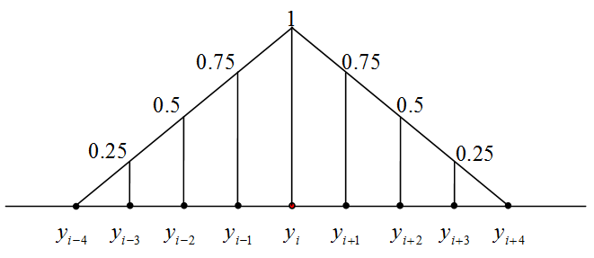
All self organizing map modification use neighborhood function to select set of nodes taking part in learning with the win nod. Neighborhood function also assign weights to nodes. In this applet Linear B-splain is used as neighborhood function.
Applet options dialog serves to assign neighborhood radius hmax (default value is equal 3). Neighborhood radius equals to 3 means three nodes before and after winner node taking part in learning (see picture).
If yi is winner node and hmax is neighborhood radius, weights of other nodes are calculated by next formula:
hij=1-|i-j|/(hmax+1) if |i-j|≤hmax and
hij=0 if |i-j|>hmax (the example is given on the left).
To use some learning algorithm (Batch SOM learning algorithm , elastic map learning algorithm, Principal tree) is necessary to associate any data points with nearest node. The set of data points associated with node yi is defined as Ci= {l:||xl-yi||2≤ ||xl-yj||2, ∀i≠j}
If for some point xl ||xl-yi|| 2=||xl-yj||2, then point xl associating with node witch has smallest number.
After association was completed we had sets {Ci}1n. The set of not associated points is empty: E=∅.
To use some learning algorithm ( Batch SOM learning algorithm , elastic map learning algorithm, Principal tree ) is necessary to associate any data points with nearest node. To use robust modification of those method is necessary to associate any data points with nearest node when distance between data point and nearest node is less or equal than robust radius. Robust radius another name is radius of data nodes interaction. The set of data points associated with node yi is defined as Ci= {l:||xl-yi||2≤ ||xl-yj||2, ||xl-yi||≤ R2, ∀i≠j}.
If for some point xl ||xl-yi|| 2=||xl-yj||2, then point xl associating with node witch has smallest number.
After association was completed we had sets {Ci}1n and set of nonassociated points E={l:||xl-yi||>R2, ∀i=1,...,n}.

|
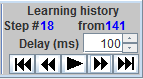
During the map learning applet saves nodes location. Every learning history record contain itself number (step number) and locations of all map nodes.
All learning history records are available to look step by step view or as slide show.
More over for this applet there exist possibilities to write history into file. If applet was started without html page as the application you can press key combinations Ctrl+P. The dialog will appear to configure output (see left).
In field select file name for history writing you have to select the file name by using button Browse.
Check box Write picture allow to switch on and of writing the picture.
Radio button group picture file format is available only if writing picture switched on. This group allow select one of the three formats to write pictures.
Radio button group Data point size is available only if eps format of file is selected.
Radio button group Write history point allow to select the frequency of output. Every step item entails the writing of all history points including steps of nodes optimizations. This option is useful for methods without growing such as SOM, EM and so on. After change number of nodes item allows to write history shortly, with fixing important states only. The states after adding or cutting the nodes and after optimization would be written. After decreasing number of nodes item is applicable for GalaPT method only. If you use cutting graph grammar, you would write history point after executing whole loop of grammars using.
The group of check boxes Write parameters allows to select parameters which would be written:
Number of nodes;
Fraction of variance unexplained (see Fraction of variance unexplained".
Energy (Lyapunov function) is applicable for elastic map and principal graphs. For SOM this parameter is not defined and would be written as zero.
Geometrical complexity is the measure of approximator complexity. For SOM and REM this value is calculated as Gc=1/4 ∑i=2, ,n-1||yi-1-2yi+ yi+1||2, for RPT this value is calculated as Gc=∑i=1, ,n,|Li|>1||yi-1/ |Li|∑j∈Liyj ||2.
Structural complexity has format number of k-stars|number of (k-1)-stars| | number of 3-stars||number of nodes. The meaning of structural complexity is described in ???.
Construction complexity is the number of grammars applications for initial graph to obtain the current graph. The meaning of construction complexity is described in ???.
Point projection on vector. |
In this applets series error of approximation evaluates as fraction of variance unexplained. Basic variance unexplained is calculated as σb=1/n ∑i=1, ,n||xi-E(x)||, E(x)= 1/n ∑i=1, ,nxi.
For given nodes {yi}1n location variance unexplained is calculated. For any data point x, its projection to map is defined. Lets node yi is nearest to point x. Node yi is connected with one (yi is outside node), two (or more for the principal tree) nodes. Lets nodes yii, ,yik are connected with node yi.
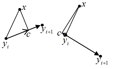
Calculate point x projection to node yi and on all edges yiyir (see left). Square of distance between node yi and point x is calculated as d0=|| x-yi||2.
To calculate point x projection on edge yiyir evaluate length of projection throw scalar product (see left): q=(x-yi ,yir-yi)/ ||yir-yi||
This value is measured in vectors (yir-yi) and may be both positive (left figure) and negative (right figure). If value q is negative, then projection on line, which contains nodes yir and yi, is out of edge yiyir. At this case define dr=∞. If value q is positive, then length of segment ||c-yi|| evaluates as is equal to q. By Pythagoras theorem distance square between point x and edge yiyir is evaluated as: dr=||c-x||2=d02- q2
Distance square between point x and other edges is evaluated analogously.
Distance square between point x and map is evaluated as Di=minr=0, ,kdr. Map variance unexplained is evaluated as σm=∑i=1, ,nDi.
Fraction of variance unexplained is evaluated as σf=σm/σb. This value is used as approximation error.
|
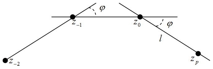
There are three nodes of broken line z-2 , z-1 , z0. Is necessary to find coordinates of new node zp such, that angle between vectors (zp -z0) and (z0 -z-1) is equal to angle between vectors (z0 -z-1) and (z-1 -z-2). Nodes z-2 , z-1 , z0 , zp form convex figure (see figure).
If nodes z-2 , z-1 , z0 is known sinφ and cosφ is evaluated as
sinφ= ((z-1,x -z-2,x )(z0,y -z-1,y )- (z-1,y -z-2,y )(z0,x -z-1,x ))/ |z-1 -z-2||z0 -z-1|.
cosφ= ((z-1,x -z-2,x )(z0,x -z-1,x )+ (z-1,y -z-2,y )(z0,y -z-1,y ))/ |z-1 -z-2||z0 -z-1|.
Unit vector along the lines (z0 -z-1) is calculated as e=(z0 -z-1)/ |z0 -z-1|.
To evaluate unit vector along the lines
(zp -z0) vector e would be multiplied by rotation matrix:
![]()
To calculate new node zp vector (zp -z0) is multiplied by l and is added to vector z0: zp=z0+l (zp -z0).
|
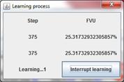
When button Learn is pressed the learning process dialog is displayed (see left). There are current number of learning steps in the first column and fraction of variance unexplained current value in the second column. Displaying data updates twice per second. If number of learning steps is changed between two last updates Learning is reflected in the bottom left corners. If number of learning steps wasnt changed during some updates Learning n is reflected, where n is number of updates.
Button Interrupt learning in the bottom right corner serves to interrupt learning process.
|
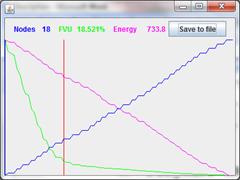
Window for graphic history reflection serves for easy visual displaying changing of some map parameters during learning process. This window accessible in universal methods GalaSOM, GalaEM, GalaPT only.
Three diagram are displayed in windows:
1. Current number of nodes
2. Fraction variance unexplained
3. Value of energy for minimization. This value is method specific.
During the history viewing red vertical line indicate current position in window. At the top of window current numerical values of parameters are displayed.
When button Save to file is pressed, following data saves to file with user specified name:
1. Step number.
2. Current quantity of nodes.
3. Fraction variance unexplained.
4. Value of energy for minimization.
File name choosing dialog is standard for using operation system.
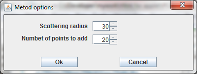
Searching radius R is parameter of this method. Fitness is evaluated as number of data points which associated with new node in accordance with "Association data points with nodes.
Searching algorithm.
1. Searching parameters is initialized as angle is zero φ=0; number of new associated points is zero nap=0; best new node is empty yp=null.
2. New node coordinates are evaluated as y0x=y1x+R cos φ, y0y=y1y+R sin φ
3. Set of new associated points is evaluated as C0={l:||xl -y0 ||≤ ||xl -yi ||, i>0}
4. If |C0|>nap, then new node is saved as best: nap=|C0|, yp=y0.
5. Angle is increased: φ=φ+20.
6. If φ<360 then go to step 2.
Searching radius R is parameter of this method. Fitness is evaluated as number of nonassociated data points which associated with new node in accordance with Robust association data points with nodes".
Searching algorithm.
1. Searching parameters is initialized as angle is zero φ=0; number of new associated points is zero nap=0; best new node is empty yp=null.
2. New node coordinates are evaluated as y0x=y1x+R cos φ, y0y=y1y+R sin φ
3. Set of new associated points is evaluated as C0={l:||xl -y0 ||≤ R , l∈E}
4. If |C0|>nap, then new node is saved as best: nap=|C0|, yp=y0.
5. Angle is increased: φ=φ+20.
6. If φ<360 then go to step 2.
Algorithm of nodes location optimization is the same for all SOM learning methods used in this applets series. All applets use Batch SOM learning algorithm.
Nodes location optimization algorithm.
1. Data points are associated with nodes ( Association data points with nodes). If used a robust modification ( GalaSOM) then would be used algorithm described in Robust association data points with nodes.
2. If all sets {Ci}1n, evaluated on step 1, are equal to sets, evaluated on previous iteration, then learning stops.
3. Add new record to learning history to place new nodes locations.
4. Centroid is calculated for every node: Xi=0 if Ci=∅ and Xi=∑j∈Cixj if Ci≠∅.
5. New location is evaluated for every node.
5.1. Following values are calculated for every node:
5.1.1. Sum weighted adjustment wci=∑j=1, ,n|Cj|hij , here |Cj| is power of set Cj or number of points associated with node yi.
5.1.2. Sum centroid Yi=∑j=1, ,nXjhij
5.2. If sum weighted adjustment is equals to zero for node yi, then new node yi location is the same as old itself location. Else new node yi location is evaluated as yi=Yi /wci.
6. Step counter is increased.
7. If step counter is equals to maximum number of optimization step, then learning stops.
8. Calculation returns to step 1.

|
There is one parameter Neighbourhood radius in Self-Organizing Map (SOM) learning algorithm. Parameter was assigned before learning start and was used to evaluate Neighborhood function.
Developed by Kohonen Batch SOM learning algorithm is used to learn.
Initial nodes location was assigned before learning start ???.
All learning steps are saved into Learning history.
If learning starts after previous learning, the last record of Learning history is used instead of user defined initial nodes location. Otherwise user defined initial nodes location is used and saved into the first learning history record.
Before learning starts sets of data points, associated with nodes, is assigned to empty set (Ci=∅, i=1, ,n), steps counter is assigned to zero. Maximum number of optimization step is assigned to 100.
Algorithm of nodes locations optimization was described in SOM nodes location optimization.
|
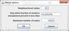
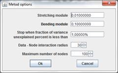
Growing Self-Organizing Map (GSOM) method is customized by following parameters assigned before learning start:
Neighbourhood radius parameter is used to evaluate Neighborhood function.
Maximum number of nodes parameter restricts size of map.
Stop when fraction of variance unexplained percent is less than parameter define threshold for fraction of variance unexplained.
Developed by Kohonen Batch SOM learning algorithm is used to learn.
Initial nodes location was assigned before learning start ???.
All learning steps are saved into Learning history.
If learning starts after previous learning, the last record of Learning history is used instead of user defined initial nodes location. Otherwise user defined initial nodes location is used and saved into the first learning history record.
Maximum number of optimization step is assigned to 20.
Map learning algorithm
1. Basic variance unexplained is calculated ( Fraction of variance unexplained).
2. Before loop starts sets of data points of associated with nodes is assigned to empty set (Ci=∅, i=1, ,n), steps counter is assigned to zero.
3. Nodes location optimization ( SOM nodes location optimization)
4. Fraction of variance unexplained fvu is evaluated.
5. If fraction of variance unexplained is less than user defined threshold then learning loop is broken off.
6. If number of nodes is equal to user defined maximum number of nodes then learning loop is broken off.
7. If user press button Interrupt learning in Learning Dialog then learning loop is broken off.
8. Map growing.
8.1. In case of map contains only one node do:
8.1.1. New node is located to place of randomly selected data point.
8.1.2. New learning history record is created. Old and new nodes are saved into record.
8.2. In case of map contains more than one node do:
8.2.1. Sets C1 and Cn is evaluated (see Association data points with nodes).
8.2.2. If those sets are empty then map growing is impossible and growing loop is broken off.
8.2.3. The first node quality is evaluated df=∑x∈C1||x-y1||2
8.2.4. The last node quality is evaluated dl=∑x∈Cn||x-yn||2
8.2.5. If df>dl, then
8.2.5.1. New nodes are created by attaching copy of the first edge to first node: y0=2y1-y2.
8.2.5.2. New set of nodes fraction of variance unexplained fvunew is evaluated.
8.2.5.3. If fvunew< fvu then new learning history record is created, new set of nodes is saved in record, learning is continued from step 2.
8.2.5.4. New node y0 is removed. New nodes are created by attaching copy of the last edge to the last node: yn+1=2yn-yn-1.
8.2.5.5. New set of nodes fraction of variance unexplained fvunew is evaluated.
8.2.5.6. If fvunew< fvu then new learning history record is created, new set of nodes is saved in record, learning is continued from step 2.
8.2.5.7. Else growing loop is broken off.
8.2.6. If df < dl, then
8.2.6.1. New nodes are created by attaching copy of the last edge to the last node: yn+1=2yn-yn-1.
8.2.6.2. New set of nodes fraction of variance unexplained fvunew is evaluated.
8.2.6.3. If fvunew< fvu then new learning history record is created, new set of nodes is saved in record, learning is continued from step 2.
8.2.6.4. New node y0 is removed. New nodes are created by attaching copy of the first edge to the first node: y0=2y1-y2.
8.2.6.5. New set of nodes fraction of variance unexplained fvunew is evaluated.
8.2.6.6. If fvunew< fvu then new learning history record is created, new set of nodes is saved in record, learning is continued from step 2.
8.2.6.7. Else growing loop is broken off.
|
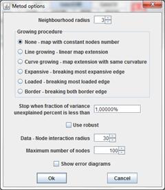
GalaSOM is universal method realizing some abilities not included to student applet. There are many options for GalaSOM.
Neighbourhood radius parameter is used to evaluate Neighborhood function.
The second parameters define growing procedure to use. Next values of this parameter available.
None map growing disabled.
Line growing map growing by adding copy of outside edges to border nodes.
Curve growing map growing by expansion with same curvature.
Expansive map growing by division most expansive edge.
Loaded map growing by division most expansive edge. Most loaded edge is edge with maximal quantity of data points associated with nodes of edge.
Border map growing by bisection outside edges.
Stop when fraction of variance unexplained percent is less than parameter define threshold for fraction of variance unexplained.
Checkbox "Use robust" switch on/off using robust version of algorithm.
Data - Node interaction radius R parameter is used to Robust association data points with nodes. This parameter also is named robust radius.
Maximum number of nodes parameter restricts size of map.
If checkbox Show error diagrams switched on, Window for graphic history reflection is displayed. There is no energy to minimize for SOM. As following this parameter not displayed in window.
Developed by Kohonen Batch SOM learning algorithm is used to learn.
Initial nodes location was assigned before learning start ???.
All learning steps are saved into Learning history.
If learning starts after previous learning, the last record of Learning history is used instead of user defined initial nodes location. Otherwise user defined initial nodes location is used and saved into the first learning history record.
Maximum number of optimization step is assigned to 20.
Map learning algorithm
1. Basic variance unexplained is calculated ( Fraction of variance unexplained).
2. Before loop starts sets of data points of associated with nodes is assigned to empty set (Ci=∅, i=1, ,n), steps counter is assigned to zero.
3. Nodes location optimization ( SOM nodes location optimization)
4. If growing procedure is None growing loop is broken off.
5. Fraction of variance unexplained fvu is evaluated.
6. If fraction of variance unexplained is less than user defined threshold then learning loop is broken off.
7. If number of nodes is equal to user defined maximum number of nodes then learning loop is broken off.
8. If user press button Interrupt learning in Learning Dialog then learning loop is broken off.
9. Map growing.
9.1. In case of map contains only one node do:
9.1.1. Lets new node is empty yp=null
9.1.2. If robust version is used and there exist nonassociated points then
9.1.2.1. Execute Robust best second node finding with r=R.
9.1.2.2. If yp=null, then execute Robust best second node finding with r=2R.
9.1.3. If yp=null, then
9.1.3.1. If robust version is used then r=R.
9.1.3.2. Else r=50.
9.1.3.3. Execute Best second node finding.
9.1.4. If yp=null, then growing is impossible and is broken off.
9.1.5. New learning history record is created. Old and new nodes are saved into record.
9.2. If number of nodes is more than one then
9.2.1. If growing procedure is Line growing or Curve growing, then
9.2.1.1. If growing procedure is "Line growing" or number of nodes is two (there is no data for expansion with save curvature), then
9.2.1.1.1. The first edge extension coefficient k is evaluated.
9.2.1.1.1.1. Lets d equal to distance between the first and the second nodes.
9.2.1.1.1.2. If robust radius is less than work desk size but greater than d, then k=R/d, else k=1.
9.2.1.1.2. New node is calculated as y0=y1+k( y1-y2).
9.2.1.1.3. The first edge extension coefficient k is evaluated.
9.2.1.1.3.1. Lets d equal to distance between the last and the penultimate nodes.
9.2.1.1.3.2. If robust radius is less than work desk size but greater than d, then k=R/d, else k=1.
9.2.1.1.4. New node is calculated as yn+1=yn+k( yn-yn-1).
9.2.1.2. If growing procedure is Curve growing and number of nodes is greater than two, then
9.2.1.2.1. The first edge extension length l is evaluated
9.2.1.2.1.1. Lets l equal to the first edge length.
9.2.1.2.1.2. If robust radius is less than work desk size but greater than l, then l=R.
9.2.1.2.2. New node y0 is calculated by executing Map extension with same curvature where z0=y1, z-1=y2, z-3=y3
9.2.1.2.3. The last edge extension length l is evaluated.
9.2.1.2.3.1. Lets l equal to the last edge length.
9.2.1.2.3.2. If robust radius is less than work desk size but greater than l, then l=R.
9.2.1.2.4. New node yn+1 is calculated by executing Map extension with same curvature where z0=yn, z-1=yn-1, z-3=yn-2
9.2.1.3. Node to expand map is selected. Lets m0=0, mn+1=0.
9.2.1.4. If there exist nonassociated data points, then m0=|{p∈E, ||xp-y0||< R}|, mn+1=|{p∈E, ||xp-yn+1||< R}|.
9.2.1.5. If m0=mn+1=0, then m0=|C0|, mn+1=|Cn+1|. Association is result of execution of Association data points with nodes.
9.2.1.6. If m0=mn+1=0, then growing is impossible and is broken off.
9.2.1.7. New learning history record is created. All old nodes is copied to created record.
9.2.1.8. If m0>0 then node y0 includes to created record.
9.2.1.9. If mn+1>0 then node yn+1 includes to created record.
9.2.2. If growing procedure is Expansive, then
9.2.2.1. New learning history record is created.
9.2.2.2. Most expansive edge defines.
9.2.2.3. New node creates in the middle of most expansive edge.
9.2.2.4. All nodes copying to created history record.
9.2.3. If growing procedure is Loaded, then
9.2.3.1. New learning history record is created.
9.2.3.2.Most loaded edge defines. Load of edge yi yi+1 is |Ci|+|Ci+1|.
9.2.3.3. New node creates in the middle of most loaded edge.
9.2.3.4. All nodes copying to created history record.
9.2.4. If growing procedure is Border, then
9.2.4.1. New learning history record is created.
9.2.4.2. All old nodes is copied to created record.
9.2.4.3. Two nodes creates in middle of the first and the last edges.
10. Go to step 2.
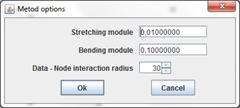
Algorithm of nodes location optimization is the same for all elastic map learning methods. This method has four parameters:
Stretching module λ
Bending module μ
Data - Node interaction radius R parameter is used to "Robust association data points with nodes". This parameter also is named robust radius.
Maximum number of optimization steps.
Nodes location optimization algorithm.
1. Data points are associated with nodes (Robust association data points with nodes). If used a not robust modification (GalaEM) use algorithm described in Association data points with nodes.
2. If all sets {Ci}1n, evaluated on step 1, are equals to sets, evaluated on previous iteration, then learning stops.
3. Add new record to learning history to place new nodes locations.
4. Centroid is calculated for every node: Xi=0 if Ci=∅ and Xi=∑j∈Cixj if Ci≠∅.
5. New location is evaluated for every node.
5.1. If map contains only one node then new node locations is evaluated as y1=X1 /|C1|
5.2. If map contain more than one node then:
5.2.1. Matrix of linear algebraic equation system is formed as sum A=A1+λA2+μA3, where matrix A1 fits with data approximation, A2 fits with edges stretching limitation, A3 fits with edges bending limitation. To form matrix following rules are used.
5.2.1.1. 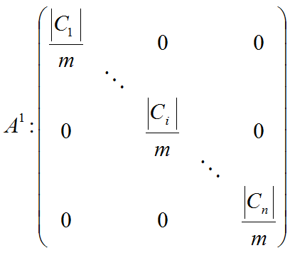
5.2.1.2. Filling in matrix A2 is depends on number of nodes.
5.2.1.2.1. In case of 2 nodes matrix is 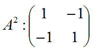
5.2.1.2.2. In case of more than 2 nodes matrix i
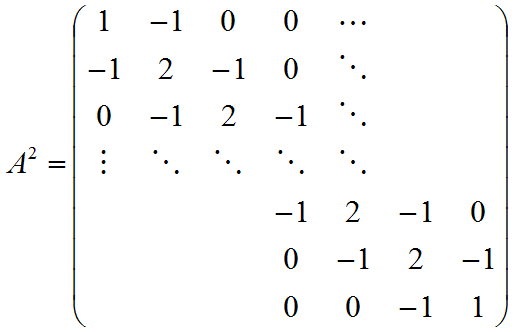
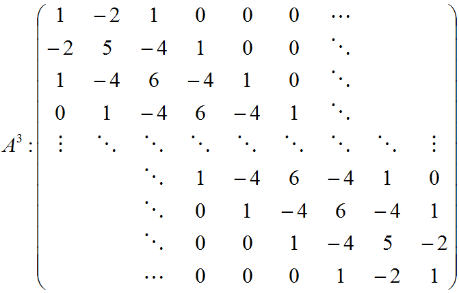
5.2.1.3. Filling in matrix A3 is depends on number of nodes.
5.2.1.3.1. In case of 2 nodes matrix A3 is zero matrix.
5.2.1.3.2. In case of 3 nodes matrix is
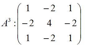
5.2.1.3.3. In case of 4 nodes matrix is
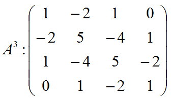
5.2.1.3.4. In case of more than 4 nodes matrix is
5.2.2. The right parts of linear algebraic equations Ay=b is bi=Xi /m
5.2.3. To solve linear algebraic equations method of Gauss elimination is used.
5.2.4. Solution of linear algebraic equations is the new map nodes locations.
6. Step counter is increased.
7. If step counter is equals to maximum number of optimization step, then learning stops.
8. Calculation returns to step 1.
|
Robust Elastic Map (REM) method is customized by following parameters assigned before learning start:
Stretching module λ
Bending module μ
Data - Node interaction radius R parameter is used to "Robust association data points with nodes". This parameter also is named robust radius. Only robust method version uses.
Initial nodes location was assigned before learning start. ???
All learning steps are saved into Learning history.
If learning starts after previous learning, the last record of Learning history is used instead of user defined initial nodes location. Otherwise user defined initial nodes location is used and saved into the first learning history record.
Before learning starts sets of data points, associated with nodes, is assigned to empty set ((Ci=∅, i=1, ,n), steps counter is assigned to zero.
To learn map Nodes location optimization for elastic map is used with maximum number of optimization step equals 100.
|
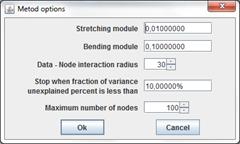
Robust Growing Elastic Map (RGEM) method is customized by following parameters assigned before learning start:
Stretching module λ
Bending module μ
Data - Node interaction radius R parameter is used to "Robust association data points with nodes". This parameter also is named robust radius. Only robust method version uses.
Maximum number of nodes parameter restricts size of map.
Stop when fraction of variance unexplained percent is less than parameter define threshold for fraction of variance unexplained.
Initial nodes location was assigned before learning start. ???
All learning steps are saved into Learning history.
If learning starts after previous learning, the last record of Learning history is used instead of user defined initial nodes location. Otherwise user defined initial nodes location is used and saved into the first learning history record.
Maximum number of optimization step is assigned to 20.
Map learning algorithm.
1. Basic variance unexplained is calculated (Fraction of variance unexplained).
2. Before loop starts sets of data points, associated with nodes, is assigned to empty set (Ci=∅, i=1, ,n), steps counter is assigned to zero.
3. Nodes location optimization (Nodes location optimization for elastic map)
4. Fraction of variance unexplained fvu is evaluated.
5. If fraction of variance unexplained is less than user defined threshold then learning loop is broken off.
6. If number of nodes is equal to user defined maximum number of nodes then learning loop is broken off.
7. Map growing
7.1. In case of map contains only one node do:
7.1.1. Lets new node is empty yp=null
7.1.2. If there exist nonassociated points then
7.1.2.1. Execute Robust best second node finding with r=R.
7.1.2.2. If yp=null, then execute Robust best second node finding with r=2R.
7.1.3. If yp=null, then r=R.
7.1.4. Execute Best second node finding.
7.1.5. If yp=null, then growing is impossible and is broken off.
7.1.6. New learning history record is created. Old and new nodes are saved into record.
7.2. In case of map contains more than one node then prepare projects to attach new adges to the first and the last nodes of map.
7.2.1. In case of map contains only two nodes linear attachments are prepared:
7.2.1.1. Edge stretching coefficient is evaluated.
7.2.1.1.1. If robust radius is less than work desk size, then k=R/||y1-y2||
7.2.1.1.2. Else k=1.
7.2.1.1.3. If k<1, then k=1.
7.2.1.2. New nodes locations are evaluated as: y0=y1+k(y1-y2), y3=y2+k(y2-y1)
7.2.2. In case of map contains more than two nodes map extension with same curvature is used.
7.2.2.1. Edge length to attach to the first node is calculated. If robust radius is less than work desk size and is more than the first edge length, then lb=R, else lb=|y2-y1|.
7.2.2.2. New first map node t0 is evaluated as Map extension with same curvature with nodes y3, y2, y1 and length lb.
7.2.2.3. Edge length to attach to the last node is calculated. If robust radius is less than work desk size and is more than the last edge length, then le=R, else le=|yn-yn-1|.
7.2.2.4. New last map node yn+1 is evaluated as Map extension with same curvature with nodes yn+2, yn+1, yn and length le.
7.2.3. Best node to expand map is chosen.
7.2.3.1. m0 and mn+1 is number of points, associated with new nodes. Let's they are zero
7.2.3.2. If nonassociated points set is not empty, values m0 and mn+1 is evaluated as: m0=|{l:l∈E, ||xl-y0||≤R}], mn+1=|{l:l∈E, ||xl-yn+1||≤R}].
7.2.3.3. In case of m0=mn+1=0, values m0 and mn+1 are evaluated as: m0=|{l:l∈E, ||xl-y0||≤||xl-yi||, i=1, ,n}], mn+1=|{l:l∈E, ||xl-yn+1||≤||xl-yi||, i=1, ,n}}].
7.2.4. If m0=mn+1=0, then growing is impossible and growing loop is broken off.
7.2.5. New history line record is created.
7.2.6. In case of m0=mn+1>0, both new nodes and old nodes are saved into learning history record.
7.2.7. In case of m0>mn+1, new node y0 and old nodes are saved into learning history record.
7.2.8. In case of m0< mn+1, new node yn+1 and old nodes are saved into learning history record.
8. Go to step 2.
|
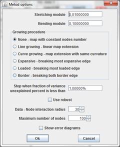
GalaEM is universal method realizing some elastic map abilities not included to student applet. There are many options for GalaEM.
Stretching module λ
Bending module μ
The third parameter define growing procedure to use. Next values of this parameter available.
None map growing disabled.
Line growing map growing by adding copy of outside edges to border nodes.
Curve growing map growing by expansion with same curvature.
Expansive map growing by division most expansive edge.
Loaded map growing by division most expansive edge. Most loaded edge is edge with maximal quantity of data points associated with nodes of edge.
Border map growing by bisection outside edges.
Stop when fraction of variance unexplained percent is less than parameter define threshold for fraction of variance unexplained.
Checkbox "Use robust" switch on/off using robust version of algorithm.
Data - Node interaction radius R parameter is used to Robust association data points with nodes. This parameter also is named robust radius.
Maximum number of nodes parameter restricts size of map.
If checkbox Show error diagrams switched on,
Window for graphic history reflection is displayed. The elastic
map energy to minimization is calculated by following formulas. If map is not
robust:
En=1/m ∑i=1,
,n∑x∈Ci
||x-yi||2+λ∑i=2,
,n||yi-yi-1||2
+μ∑i=2,
,n-1||yi-1-2yi+yi+1||2
If map is robust:
En=1/m (∑i=1,
,n∑x∈Ci
||x-yi||2+|E|R2)
+λ∑i=2,
,n||yi-yi-1||2
+μ∑i=2,
,n-1||yi-1-2yi+yi+1||2
Initial nodes location was assigned before learning start ???.
All learning steps are saved into Learning history.
If learning starts after previous learning, the last record of Learning history is used instead of user defined initial nodes location. Otherwise user defined initial nodes location is used and saved into the first learning history record.
Maximum number of optimization step is assigned to 20.
Map learning algorithm
1. Basic variance unexplained is calculated ( Fraction of variance unexplained).
2. Before loop starts sets of data points of associated with nodes is assigned to empty set (Ci=∅, i=1, ,n), steps counter is assigned to zero.
3. Nodes location optimization ( Nodes location optimization for elastic map)
4. If growing procedure is None growing loop is broken off.
5. Fraction of variance unexplained fvu is evaluated.
6. If fraction of variance unexplained is less than user defined threshold then learning loop is broken off.
7. If number of nodes is equal to user defined maximum number of nodes then learning loop is broken off.
8. If user press button Interrupt learning in Learning Dialog then learning loop is broken off.
9. Map growing.
9.1. In case of map contains only one node do:
9.1.1. Lets new node is empty yp=null
9.1.2. If robust version is used and there exist nonassociated points then
9.1.2.1. Execute Robust best second node finding with r=R.
9.1.2.2. If yp=null, then execute Robust best second node finding with r=2R.
9.1.3. If yp=null, then
9.1.3.1. If robust version is used then r=R.
9.1.3.2. Else r=50.
9.1.3.3. Execute Best second node finding.
9.1.4. If yp=null, then growing is impossible and is broken off.
9.1.5. New learning history record is created. Old and new nodes are saved into record.
9.2. If number of nodes is more than one then
9.2.1. If growing procedure is Line growing or Curve growing, then
9.2.1.1. If growing procedure is "Line growing" or number of nodes is two (there is no data for expansion with save curvature), then
9.2.1.1.1. The first edge extension coefficient k is evaluated.
9.2.1.1.1.1. Lets d equal to distance between the first and the second nodes.
9.2.1.1.1.2. If robust radius is less than work desk size but greater than d, then k=R/d, else k=1.
9.2.1.1.2. New node is calculated as y0=y1+k( y1-y2).
9.2.1.1.3. The first edge extension coefficient k is evaluated.
9.2.1.1.3.1. Lets d equal to distance between the last and the penultimate nodes.
9.2.1.1.3.2. If robust radius is less than work desk size but greater than d, then k=R/d, else k=1.
9.2.1.1.4. New node is calculated as yn+1=yn+k( yn-yn-1).
9.2.1.2. If growing procedure is Curve growing and number of nodes is greater than two, then
9.2.1.2.1. The first edge extension length l is evaluated
9.2.1.2.1.1. Lets l equal to the first edge length.
9.2.1.2.1.2. If robust radius is less than work desk size but greater than l, then l=R.
9.2.1.2.2. New node y0 is calculated by executing Map extension with same curvature where z0=y1, z-1=y2, z-3=y3
9.2.1.2.3. The last edge extension length l is evaluated.
9.2.1.2.3.1. Lets l equal to the last edge length.
9.2.1.2.3.2. If robust radius is less than work desk size but greater than l, then l=R.
9.2.1.2.4. New node yn+1 is calculated by executing Map extension with same curvature where z0=yn, z-1=yn-1, z-3=yn-2
9.2.1.3. Node to expand map is selected. Lets m0=0, mn+1=0.
9.2.1.4. If there exist nonassociated data points, then m0=|{p∈E, ||xp-y0||< R}|, mn+1=|{p∈E, ||xp-yn+1||< R}|.
9.2.1.5. If m0=mn+1=0, then m0=|C0|, mn+1=|Cn+1|. Association is result of execution of Association data points with nodes.
9.2.1.6. If m0=mn+1=0, then growing is impossible and is broken off.
9.2.1.7. New learning history record is created. All old nodes is copied to created record.
9.2.1.8. If m0>0 then node y0 includes to created record.
9.2.1.9. If mn+1>0 then node yn+1 includes to created record.
9.2.2. If growing procedure is Expansive, then
9.2.2.1. New learning history record is created.
9.2.2.2. Most expansive edge defines.
9.2.2.3. New node creates in the middle of most expansive edge.
9.2.2.4. All nodes copying to created history record.
9.2.3. If growing procedure is Loaded, then
9.2.3.1. New learning history record is created.
9.2.3.2.Most loaded edge defines. Load of edge yi yi+1 is |Ci|+|Ci+1|.
9.2.3.3. New node creates in the middle of most loaded edge.
9.2.3.4. All nodes copying to created history record.
9.2.4. If growing procedure is Border, then
9.2.4.1. New learning history record is created.
9.2.4.2. All old nodes is copied to created record.
9.2.4.3. Two nodes creates in middle of the first and the last edges.
10. Go to step 2.
All principal tree methods uses nodes location optimization procedure in some place of algorithms. Abstraction this procedure is needed. Nodes location optimization procedure parameters is listed below.
Stretching module λ
Bending module μ
Scaling exponent α
Necessity to save optimization history.
Optimization algorithm
1. Data points are associated with nodes
1.1. If used a non robust modification Association data points with nodes executed.
1.2. If used a robust modification Robust association data points with nodes executed.
2. If all sets {Ci}1n is empty then algorithm stops.
3. If all sets {Ci}1n, evaluated on step 1, are equals to sets, evaluated on previous iteration, then learning stops.
4. Step counter is increased.
5. If step counter is equals to maximum number of optimization step, then learning stops.
6. If save history is necessary, add new record of learning history to place new nodes locations is created, else pseudo history record is created.
7. Centroids are calculated for every node: Xi=0 if Ci=∅ and Xi=∑j∈Cixj if Ci≠∅.
8. New location is evaluated for every node.
8.1. If map contains only one node then new node locations is evaluated as y1=X1 /|C1|
8.2. If map contain more than one node then:
8.2.1. Matrix of linear algebraic equation system is formed as sum A=A1+λA2+μA3, where matrix A1 fits with data approximation, A2 fits with edges stretching limitation, A3 fits with edges bending limitation. To form matrix following rules are used.
8.2.1.1.
8.2.1.2. Filling in matrix A2 is calculated by next algorithm.
8.2.1.2.1. Let's all elements of matrix A2 are zero aij2=0.
8.2.1.2.2. For any node yi execute next procedure. For any j∈Li, j>i do next changes in matrix A2
8.2.1.2.2.1. aii2←aii2+1
8.2.1.2.2.2. ajj2←ajj2+1
8.2.1.2.2.3. aij2←aij2-1
8.2.1.2.2.4. aji2←aji2-1
8.2.1.3. Matrix A3 is calculated by next algorithm.
8.2.1.3.1. Let's all elements of matrix A2 are zero aij3=0.
8.2.1.3.2. For any node yi with |Li|>1 execute next procedure
8.2.1.3.2.1. The diagonal element is changed as aii3←aii3+|Li|α
8.2.1.3.2.2. Following elements of i-th row is changed for any j∈Li: aij3←aij3-|Li|α-1
8.2.1.3.2.3. Following elements of j-th row is changed for any j∈Li:
8.2.1.3.2.3.1. aji3←aji3-|Li|α-1
8.2.1.3.2.3.2. Following elements of j-th row is changed for any k∈Li: ajk3←ajk3-|Li|α-2
8.2.2. The right parts of linear algebraic equations Ay=b is bi=Xi /m
8.2.3. To solve linear algebraic equations method of Gauss elimination is used.
8.2.4. Solution of linear algebraic equations is the new map nodes locations.
9. Calculation returns to step 1.
|
Robust principal tree (topological grammar) method uses growing grammar only. Method has following parameters.
Stretching module λ
Bending module μ
Data - Node interaction radius R parameter is used to Robust association data points with nodes. This parameter also is named robust radius.
Stop when fraction of variance unexplained percent is less than parameter define threshold for fraction of variance unexplained.
Maximum number of nodes parameter restricts size of map.
Initial nodes location was assigned before learning start ???.
All learning steps are saved into Learning history.
If learning starts after previous learning, the last record of Learning history is used instead of user defined initial nodes location. Otherwise user defined initial nodes location is used and saved into the first learning history record.
Nodes location optimization for principal tree is used on some algorithms steps. This method used robust version only. Scaling exponent sets to zero. Maximum number of optimization step is assigned to 20.
The principal tree energy to minimization is calculated as En=1/m (∑i=1, ,n∑x∈Ci ||x-yi||2+|E|R2) +λ∑i=1, ,n∑j∈Li, j>i||yi-yj||2 +μ∑i=1, ,n, |Li|>1 ||yi-1/|Li| ∑j∈Liyj||2
Tree learning algorithm.
1. Basic variance unexplained is calculated ( Fraction of variance unexplained).
2. Nods optimization with history saving executes.
3. Fraction of variance unexplained fvu is evaluated.
4. If fraction of variance unexplained is less than user defined threshold then learning loop is broken off.
5. If number of nodes is equal to user defined maximum number of nodes then learning loop is broken off.
6. If user press button Interrupt learning in Learning Dialog then learning loop is broken off.
7. Loop of tree structure changing.
7.1. In case of map contains only one node do:
7.1.1. Lets new node is empty yp=null
7.1.2. If there exist nonassociated points then
7.1.2.1. Execute Robust best second node finding with r=R.
7.1.2.2. If yp=null, then execute Robust best second node finding with r=2R.
7.1.3. If yp=null, then r=R, execute Best second node finding.
7.1.4. If yp=null, then growing is impossible and is broken off.
7.1.5. New learning history record is created. Old and new nodes are saved into record.
7.2. If number of nodes is more than one then
7.2.1. Optimal energy value sets to ∞, rule number sets to zero, best node number sets to zero.
7.2.2. Add node and edge rule using. Next procedure executes for any node yi.
7.2.2.1. New node adds to node yi with zero flexible energy of new node yi star: ynew=(|Li|+1)yi-∑j∈Liyi
7.2.2.2. Nods optimization without history saving executes.
7.2.2.3. Minimizing energy value is evaluated for the step 7.2.2.2 result tree.
7.2.2.4. If evaluated minimizing energy value is less than optimal energy value then optimal energy value sets to evaluated minimizing energy value, best node number sets to i, rule number sets to 1.
7.2.3. Add node by edge cutting rule using. Next procedure executes for any edge:
7.2.3.1. New node adds to middle of edge.
7.2.3.2. Nods optimization without history saving executes.
7.2.3.3. Minimizing energy value is evaluated for the step 8.2.2.2.2 result tree.
7.2.3.4. If evaluated minimizing energy value is less than optimal energy value then optimal energy value sets to evaluated minimizing energy value, best nodes numbers sets to nodes of edge, rule number sets to 2.
7.2.4. New learning history record is created.
7.2.5. If rule number is 1, then best node is added. Old and new nodes are saved into record.
7.2.6. If rule number is 2, then new node add to middle of best nodes edge. Old and new nodes are saved into record.
8. Go to step 2
|
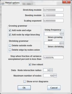
GalaPT is the principal tree (topological grammar) universal method, included many abilities excluded from student applet. GalaPT has many parameters.
Stretching module λ
Bending module μ
Scaling exponent α
The third parameters Scaling exponent α define factor in Nodes location optimization for principal tree and energy for minimization.
Growing grammar group of checkboxes is define growing grammar rules to use.
Checkbox Add node and edge switches on/off using of adding new node to existing node rule.
Checkbox Add node by edge cutting switches on/off using of division edges rule.
Shrinking grammar group of checkboxes is define shrinking grammar rules to use.
Checkbox Delete outside node switches on/off using of removing outside node rule.
Checkbox Delete edge by nodes union switches on/off using of edge removing rule. When edge is removed its nodes (stars) is united.
The Using frequency fields group serves to control using growing grammar and shrinking grammar frequency. At every loop the first do some (upper field) steps of growing grammar, then some (down field) steps of shrinking grammar.
Stop when fraction of variance unexplained percent is less than parameter define threshold for fraction of variance unexplained.
Checkbox «Use robust» switch on/off using robust version of algorithm.
Data - Node interaction radius R parameter is used to Robust association data points with nodes. This parameter also is named robust radius.
Maximum number of nodes parameter restricts size of map.
If checkbox Show error diagrams switched on, Window for graphic history reflection is displayed.
The principal tree energy to minimization is calculated by following formulas. If tree is not robust:
En=1/m ∑i=1,
,n∑x∈Ci||x-yi||2
+λ∑i=1,
,n∑j∈Li, j>i||yi-yj||
2+μ∑i=1,
,n, |Li|>1
||yi-1/|Li| ∑j∈Liyj||2
If tree is robust
En=1/m (∑i=1,
,n∑x∈Ci
||x-yi||2+|E|R2)
+λ∑i=1,
,n∑j∈Li, j>i||yi-yj||
2
+μ∑i=1,
,n, |Li|>1
||yi-1/|Li| ∑j∈Liyj||2
Initial nodes location was assigned before learning start ???.
All learning steps are saved into Learning history.
If learning starts after previous learning, the last record of Learning history is used instead of user defined initial nodes location. Otherwise user defined initial nodes location is used and saved into the first learning history record.
Maximum number of optimization step is assigned to 20.
Tree learning algorithm
1. Basic variance unexplained is calculated ( Fraction of variance unexplained).
2. Growing indicator is set to true (the growing rules executed the first). Tree changing operation number is set to user defined growing grammar steps.
3. Nods optimization with history saving executes.
4. Fraction of variance unexplained is evaluated.
5. If fraction of variance unexplained is less than user defined threshold then learning loop is broken off.
6. If number of nodes is equal to user defined maximum number of nodes then learning loop is broken off.
7. If user press button Interrupt learning in Learning Dialog then learning loop is broken off.
8. Loop of tree structure changing
8.1. In case of map contains only one node do:
8.1.1. Lets new node is empty yp=null
8.1.2. If robust version is used and there exist nonassociated points then
8.1.2.1. Execute Robust best second node finding with r=R.
8.1.2.2. If yp=null, then execute Robust best second node finding with r=2R.
8.1.3. If yp=null, then
8.1.3.1. If robust version is used then r=R.
8.1.3.2. Else r=50.
8.1.3.3. Execute Best second node finding
8.1.4. If yp=null, then growing is impossible and is broken off.
8.1.5. New learning history record is created. Old and new nodes are saved into record.
8.2. If number of nodes is more than one then
8.2.1. Optimal energy value sets to ∞, rule number sets to zero, best node number sets to zero.
8.2.2.If growing indicator is true, then
8.2.2.1. If checkbox Add node and edge is switched on, then next procedure executes for any node yi.
8.2.2.1.1. New node adds to node yi with zero flexible energy of new node yi star: ynew=(|Li|+1)yi-∑j∈Liyi
8.2.2.1.2. Nods optimization without history saving executes.
8.2.2.1.3. Minimizing energy value is evaluated for the step 8.2.2.1.2 result tree.
8.2.2.1.4. If evaluated minimizing energy value is less than optimal energy value then optimal energy value sets to evaluated minimizing energy value, best node number sets to i, rule number sets to 1.
8.2.2.2. If checkbox Add node by edge cutting is switched on, then next procedure executes for any edge:
8.2.2.2.1. New node adds to middle of edge.
8.2.2.2.2. Nods optimization without history saving executes.
8.2.2.2.3. Minimizing energy value is evaluated for the step 8.2.2.2.2 result tree.
8.2.2.2.4. If evaluated minimizing energy value is less than optimal energy value then optimal energy value sets to evaluated minimizing energy value, best nodes numbers sets to nodes of edge, rule number sets to 2.
8.2.2.3. New learning history record is created.
8.2.2.4. If rule number is 1, then best node is added. Old and new nodes are saved into record.
8.2.2.5. If rule number is 2, then new number add to middle of best nodes edge. Old and new nodes are saved into record.
8.2.3. If growing indicator is false, then
8.2.3.1. If checkbox Delete outside node is switched on, then next procedure executes for any nodes with |Li|=1
8.2.3.1.1. The yi node removes.
8.2.3.1.2. Nods optimization without history saving executes.
8.2.3.1.3. Minimizing energy value is evaluated for the step 8.2.3.1.2 result tree.
8.2.3.1.4. If evaluated minimizing energy value is less than optimal energy value then optimal energy value sets to evaluated minimizing energy value, best nodes numbers sets to i, rule number sets to 3.
8.2.3.2. If checkbox Delete edge by nodes union is switched on, then next procedure executes for any edge connects not outside nodes yi and yj (∀i≠j):
8.2.3.2.1. All nodes connected with yj connects with yi. The yj node removes.
8.2.3.2.2. Nods optimization without history saving executes.
8.2.3.2.3. Minimizing energy value is evaluated for the step 8.2.3.2.2 result tree.
8.2.3.2.4. If evaluated minimizing energy value is less than optimal energy value then optimal energy value sets to evaluated minimizing energy value, best nodes numbers sets to nodes of edge, rule number sets to 4.
8.2.3.3. New learning history record is created.
8.2.3.4. If rule number is 3, then best node removes. Kept nodes are copied into record.
8.2.3.5. If rule number is 4, then best nodes edge removes. Kept nodes are copied into record.
8.2.4. Tree changing operations number is decreased by 1. If it equals zero, then
8.2.4.1. Growing indicator is set to not growing indicator.
8.2.4.2. If growing indicator is true, tree changing operation number is set to user defined growing grammar steps.
8.2.4.3. If growing indicator is false, tree changing operation number is set to user defined shrinking grammar steps.
8.2.4.4. If tree changing operation number equals to zero (it is possible, when user defined shrinking grammar steps equals to zero), growing indicator is set to true, tree changing operation number is set to user defined growing grammar steps.
9. Go to step 3
The applet contains several menu panels (top left), the University of Leicester label (top right), work desk (center) and the label of the Attribution 3.0 Creative Commons publication license (bottom).
To wisit the web-site of the University of Leicester click on the University of Leicester logo.
To read the Creative Commons publication license click on the bottom license panel.
|
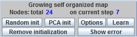
Common parts of the menu panel for all methods
The All methods menu panel containes two parts.
|
|

|
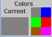
For PCA, all points and lines are in a blue color. The points for PCA have the form of four-ray stars (see left). To start PCA learning two points are needed. You can select initial points by mouse clicks at choosen locations, or by the button Random initialization. When you try add the third point, the first point is removed.
After learning is finished, use the Learning history buttons at the right part of menu panel to look at the learning history and results. You will see one four-ray star, the centroid of the data set, and one line, the current approximation of the first principal component.

|
For SOM, all points and lines are in a red color. The points for SOM have the square form (see left). To start SOM learning, the initial positions of all coding vectors are needed. To add a point to an initial approximation, click the mouse button at the choosen location, or use the button Random init or the button PCA init. When you add a new point, it is attached to the last added point.
After learning is finished, use the Learning history buttons at the right part of menu panel to look at the learning history and results.

|
For GSOM, all points and lines are in a brown color. The points for GSOM have the square form (see left). To start learning, GSOM is needed to initiate one point. To place initial point click the mouse button in the chosen location, or push the button Random init or the button PCA init. When you add a new point, the new point is joined with the last added point.
After learning is finished, use the Learning history buttons at the right part of menu panel to look at the learning history and results.

|
For GalaSOM, all points and lines are in a green color. The points for GalaSOM have the square form (see left). To start learning, GalaSOM is needed to initiate one point. To place initial point click the mouse button in the chosen location, or push the button Random init or the button PCA init. When you add a new point, the new point is joined with the last added point.
After learning is finished, use the Learning history buttons at the right part of menu panel to look at the learning history and results.

|
For REM, all points and lines are in a red color. The points for SOM have the form of triangle (see left). To start REM learning, the initial positions of all coding vectors are needed. To add a point to an initial approximation, click the mouse button at the choosen location, or use the button Random init or the button PCA init. When you add a new point, it is attached to the last added point.
After learning is finished, use the Learning history buttons at the right part of menu panel to look at the learning history and results.

|
For RGEM, all points and lines are in a brown color. The points for GalaSOM have the form of triangle (see left). To start learning, RGEM is needed to initiate one point. To place initial point click the mouse button in the chosen location, or push the button Random init or the button PCA init. When you add a new point, the new point is joined with the last added point.
After learning is finished, use the Learning history buttons at the right part of menu panel to look at the learning history and results.

|
For GalaEM, all points and lines are in a green color. The points for GalaSOM have the form of triangle (see left). To start learning, GalaEM is needed to initiate one point. To place initial point click the mouse button in the chosen location, or push the button Random init or the button PCA init. When you add a new point, the new point is joined with the last added point.
After learning is finished, use the Learning history buttons at the right part of menu panel to look at the learning history and results.
|
|
For RPT, all points and lines are in a brown color. The points for GalaSOM have the form of circle (see left). To start learning, RPT is needed to initiate one point. To place initial point click the mouse button in the chosen location, or push the button Random init or the button PCA init. When you add a new point, the new point is joined with the last added point.
After learning is finished, use the Learning history buttons at the right part of menu panel to look at the learning history and results.
|
|
For GalaPT, all points and lines are in a green color. The points for GalaSOM have the form of circle (see left). To start learning, GalaPT is needed to initiate one point. To place initial point click the mouse button in the chosen location, or push the button Random init or the button PCA init. When you add a new point, the new point is joined with the last added point.
After learning is finished, use the Learning history buttons at the right part of menu panel to look at the learning history and results.
|